5  SWaT PIT-502 Pressure Sensor: A Real-World Example

This example applies change-point detection to the PIT-502 pressure sensor in the Secure Water Treatment (SWaT) dataset.

5.1 Load the Data

library(scanr)

Load the dataset and resample it at one-minute intervals for change-point detection.

head(swat)

               Timestamp   PIT502 Normal/Attack
1 28/12/2015 10:00:00 AM 1.649953        Normal
2 28/12/2015 10:01:00 AM 1.649953        Normal
3 28/12/2015 10:02:00 AM 1.665972        Normal
4 28/12/2015 10:03:00 AM 1.681991        Normal
5 28/12/2015 10:04:00 AM 1.746067        Normal
6 28/12/2015 10:05:00 AM 1.681991        Normal

5.2 Choose Window Sizes

The largest candidate window is \(\lfloor n^{2/3}\rfloor\). The package helper selects 15 default window sizes between 20 minutes and that upper bound.

n <- nrow(swat)
window_sizes <- scanr::default_window_sizes(
  n,
  min_window = 100,
  max_window = floor(n^(2 / 3)),
  n_windows = 10,
  seed = 400
)
window_sizes

 [1] 201 255 426 442 519 587 607 624 625 652

The PIT-502 measurements are standardized before detection. Standardization changes their units but preserves the locations of mean shifts.

x <- as.numeric(scale(swat[["PIT502"]]))

5.3 Detect change-points

The R interface uses n_boot and random_state for bootstrap calibration and reproducibility.

fit_swat <- scan_cpd(
  x,
  window_sizes = window_sizes,
  n_boot = 400,
  vote_threshold = 0.15,
  random_state = 100,
  change_type = "mean",
  n_jobs = -1
)

fit_swat

scanr change-point result
observations: 17477 
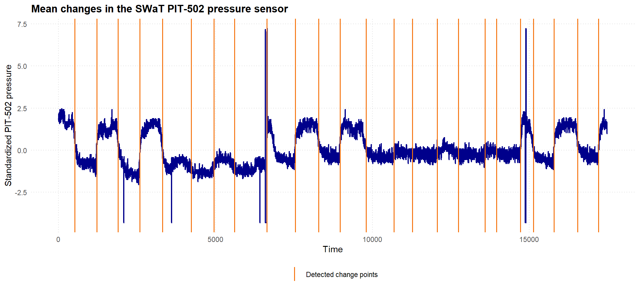
change points: 517, 1222, 1901, 2596, 3311, 4232, 4952, 5610, 6643, 7542, 8291, 8972, 9799, 10689, 11277, 12063, 12741, 13588, 13960, 14718, 15131, 15792, 16541, 17201 

The fitted object stores change points as positions in the one-minute series. We can map those positions back to timestamps, observed pressures, and the dataset’s operating-state labels.

detected_changes <- swat[
  fit_swat$change_points,
  c("Timestamp", "PIT502", "Normal/Attack"),
  drop = FALSE
]

cat("Number of change-points:", nrow(detected_changes), "\n")

Number of change-points: 24 

5.4 Visualize the Result

vis_change_points(
  x,
  fit_swat,
  index = seq_along(x),
  x_label = "Time",
  y_label = "Standardized PIT-502 pressure",
  title = "Mean changes in the SWaT PIT-502 pressure sensor"
)

5.5 Inspect the Vote Scree

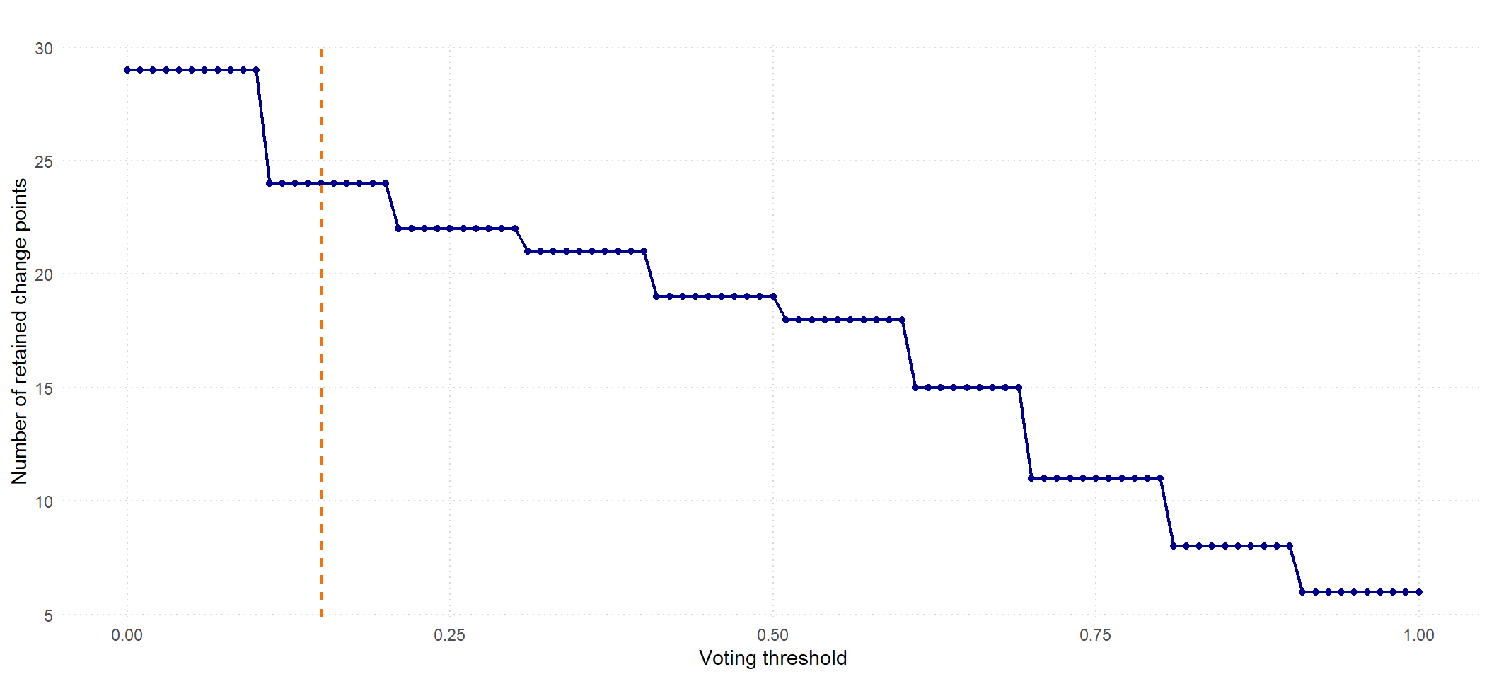
The vote scree shows how much support each candidate location receives across the selected window sizes. The horizontal threshold corresponds to the vote_threshold = 0.15 used above.

vis_vote_scree(fit_swat)