4  Change in Distribution (Example 2)

This example uses segments from different distribution families, including normal, exponential, Poisson, gamma, uniform, Student’s t, lognormal, beta, Weibull, and chi-square distributions. Each segment is standardized before being rescaled, so the signal is not only a simple shift in the mean. This creates a more challenging distributional change-point problem.

set.seed(1234)

n <- 20000

change_points <- c(
  952, 1905, 2858, 3810, 4763, 5715, 6668, 7620, 8573, 9525,
  10478, 11430, 12383, 13335, 14288, 15240, 16193, 17145, 18098,
  19050
)

segment_starts <- c(1, change_points + 1)
segment_ends <- c(change_points, n)

families <- c(
  "normal", "exponential", "poisson", "t", "gamma", "uniform", "lognormal",
  "weibull", "chisq", "beta", "normal", "poisson", "exponential", "uniform",
  "gamma", "t", "lognormal", "beta", "weibull", "chisq", "normal"
)

scale_factors <- c(
  0.7, 1.4, 0.6, 1.8, 0.75, 2.5, 0.65, 3.0, 0.7, 2.6, 0.6,
  1.7, 0.65, 2.9, 0.7, 2.8, 0.6, 2.6, 0.65, 3.0, 0.7
)

simulate_base <- function(m, family) {
  z <- switch(
    family,
    normal = rnorm(m, mean = 0, sd = 1),
    exponential = rexp(m, rate = 1),
    poisson = rpois(m, lambda = 2),
    gamma = rgamma(m, shape = 2, rate = 1),
    uniform = runif(m, min = -sqrt(3), max = sqrt(3)),
    t = rt(m, df = 3),
    lognormal = rlnorm(m, meanlog = 0, sdlog = 0.7),
    beta = rbeta(m, shape1 = 2, shape2 = 5),
    weibull = rweibull(m, shape = 1.5, scale = 1),
    chisq = rchisq(m, df = 5)
  )
  as.numeric((z - mean(z)) / sd(z))
}

x_dist <- numeric(n)

for (j in seq_along(families)) {
  segment_index <- segment_starts[j]:segment_ends[j]
  x_dist[segment_index] <- scale_factors[j] * simulate_base(length(segment_index), families[j])
}

change_points

 [1]   952  1905  2858  3810  4763  5715  6668  7620  8573  9525 10478 11430
[13] 12383 13335 14288 15240 16193 17145 18098 19050

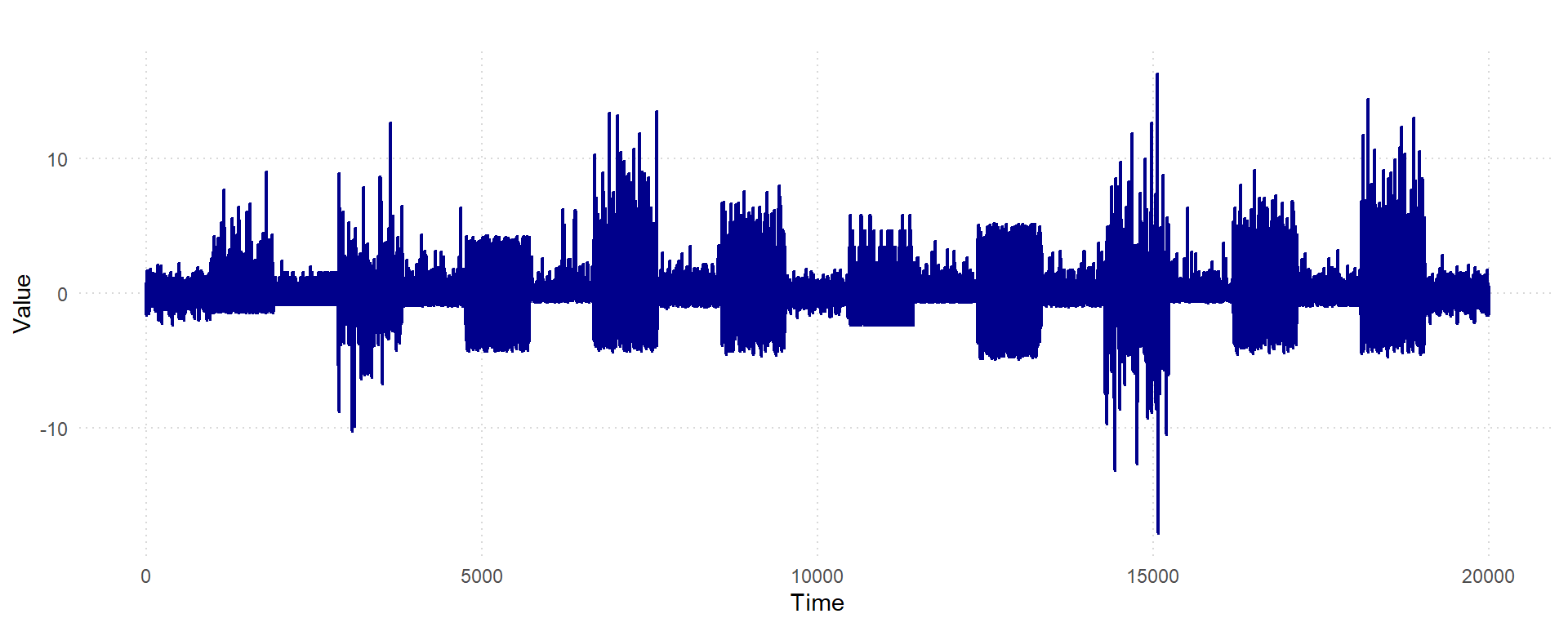
The simulated series contains changes in distributional shape and scale.

4.1 Run SCAN Change-Point Detection

For distributional changes, set change_type = "distribution". This uses the distribution-sensitive local statistic rather than a mean-only statistic.

window_sizes <- default_window_sizes(
  length(x_dist),
  min_window = 100L,
  max_window = floor(length(x_dist)^(2 / 3)),
  n_windows = 15L
)

fit_dist <- scan_cpd(
  x_dist,
  window_sizes = window_sizes,
  n_boot = 1000,
  random_state = 1234,
  change_type = "distribution",
  vote_threshold = 0.5,
  n_jobs = 1
)

The set of estimated change points is:

fit_dist$change_points

 [1]   954  1902  2860  3809  4764  5709  6669  7611  8573  9522 10478 11430
[13] 12383 13335 14289 15240 16195 17145 18100 19048

4.2 Evaluate Detection Accuracy

cpd_metrics(
  true_cps = change_points,
  estimated_cps = fit_dist$change_points,
  n = length(x_dist),
  tolerance = 20
)

$matches
    true estimated distance
1   8573      8573        0
2  10478     10478        0
3  11430     11430        0
4  12383     12383        0
5  13335     13335        0
6  15240     15240        0
7  17145     17145        0
8   3810      3809        1
9   4763      4764        1
10  6668      6669        1
11 14288     14289        1
12   952       954        2
13  2858      2860        2
14 16193     16195        2
15 18098     18100        2
16 19050     19048        2
17  1905      1902        3
18  9525      9522        3
19  5715      5709        6
20  7620      7611        9

$precision
[1] 1

$recall
[1] 1

$f1
[1] 1

$covering
[1] 0.9965096

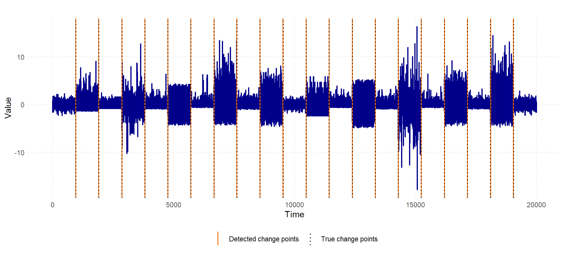
4.3 Visualize the Result

vis_change_points(
  x_dist,
  fit_dist,
  true_change_points = change_points,
  x_label = "Time",
  y_label = "Value"
)