6  SWAL Statistic for Single Change-Point Detection

The SCAN procedure above combines local evidence across many windows. The package also exposes lower-level localization tools for a single region that is believed to contain one change point.

For a mean change, the mean version of the SWAL statistic aligns with the CUSUM localizer. Both methods search for the split that best separates the left and right sides of the local region.

set.seed(1234)

true_single_cp <- 150
mean_region <- c(
  rnorm(true_single_cp, mean = 0, sd = 1),
  rnorm(true_single_cp, mean = 2, sd = 1)
)

c(
  truth = true_single_cp,
  cusum = ts_cusum(mean_region),
  swal_distribution = swal_statistic(mean_region, change_type = "distribution")
)

            truth             cusum swal_distribution 
              150               150               150 

The distributional version is more general. It can localize changes where the mean is approximately unchanged but other aspects of the distribution, such as variance, change sharply. In the example below, both segments have mean zero, but the second segment has a much larger standard deviation.

set.seed(1234)

var_region <- c(
  rnorm(true_single_cp, mean = 0, sd = 0.5),
  rnorm(true_single_cp, mean = 0, sd = 2)
)

c(
  truth = true_single_cp,
  cusum = ts_cusum(var_region),
  swal_distribution = swal_statistic(var_region, change_type = "distribution")
)

            truth             cusum swal_distribution 
              150               164               152 

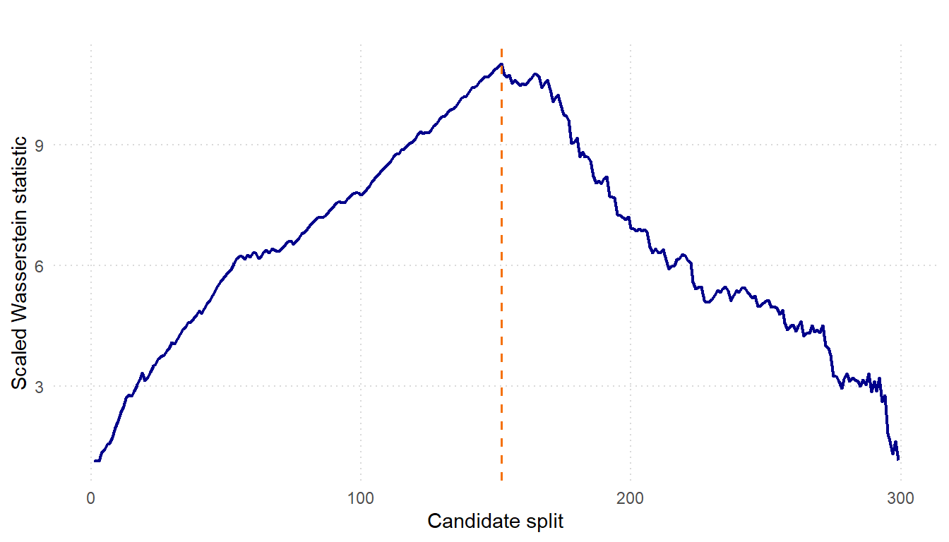
The ts_wasserstein() function returns both the estimated split and the full sequence of split statistics. The plotting helper vis_swal_curve() displays that localization curve, making it easier to inspect where the statistic is maximized.

vis_swal_curve(
  var_region,
  start = 1,
  end = length(var_region),
  x_label = "Candidate split",
  y_label = "Scaled Wasserstein statistic",
  title = ""
)