3 Change in Mean (Example 1)

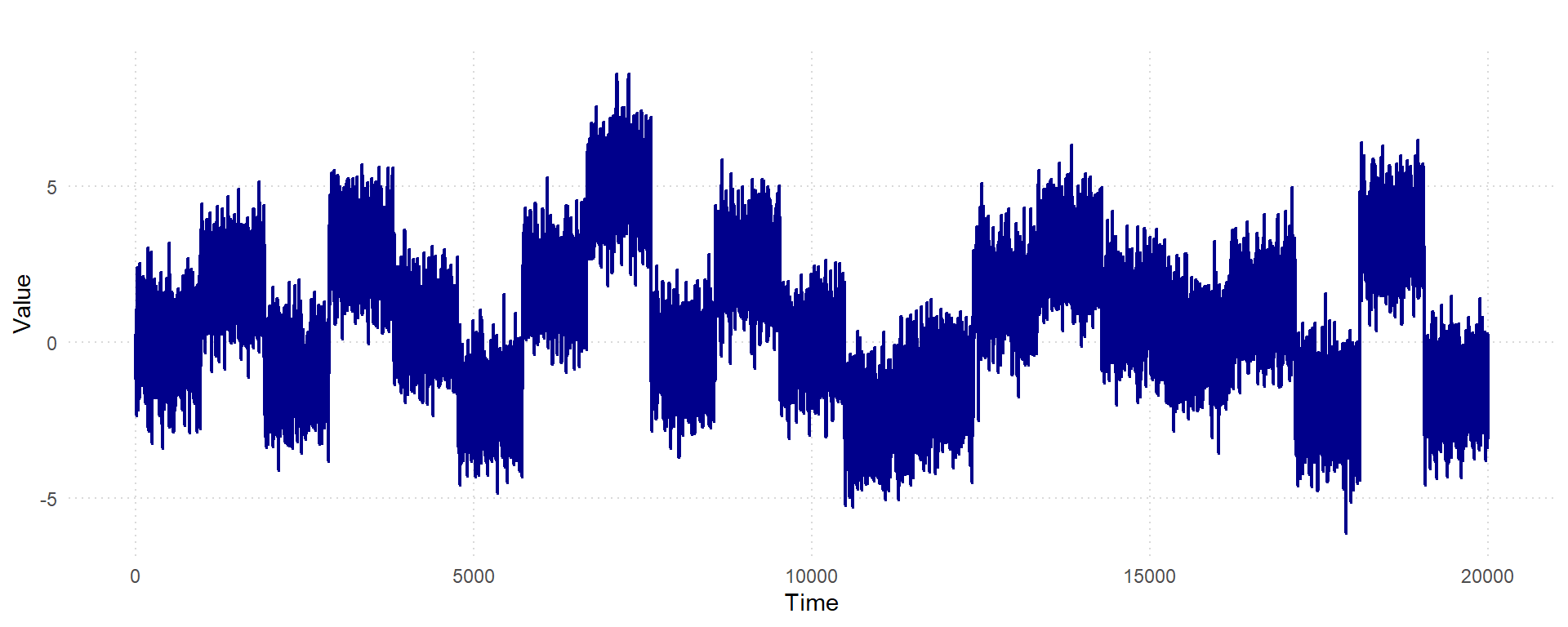
We first simulate a white-noise time series of length 20,000 with 20 change points and 21 piecewise-constant mean regimes. The noise variance is fixed, so this example focuses on changes in the mean.

set.seed(1234)

n <- 20000

change_points <- c(
  952, 1905, 2858, 3810, 4763, 5715, 6668, 7620, 8573, 9525,
  10478, 11430, 12383, 13335, 14288, 15240, 16193, 17145, 18098,
  19050
)

means <- c(
  0, 2, -1, 3, 0.5, -2, 2, 5, -0.5, 2.5, 0, -2.5, -1.5, 1.5,
  3, 1, 0, 1.25, -2, 3.5, -1.5
)

segment_starts <- c(1L, change_points + 1L)
segment_ends <- c(change_points, n)
x_mean <- numeric(n)

for (j in seq_along(means)) {
  segment_index <- segment_starts[j]:segment_ends[j]
  x_mean[segment_index] <- rnorm(length(segment_index), mean = means[j], sd = 1)
}

change_points

 [1]   952  1905  2858  3810  4763  5715  6668  7620  8573  9525 10478 11430
[13] 12383 13335 14288 15240 16193 17145 18098 19050

The plot below shows the simulated series.

3.1 Run SCAN Change-Point Detection

The window_sizes argument controls the local scales used by the scan. The window sizes should be smaller than the spacing between nearby change points, while still being large enough to estimate the local distributions on each side of a candidate split.

window_sizes <- default_window_sizes(
  length(x_mean),
  min_window = 100L,
  max_window = floor(length(x_mean)^(2 / 3)),
  n_windows = 11L
)

fit_mean <- scan_cpd(
  x_mean,
  window_sizes = window_sizes,
  n_boot = 400,
  random_state = 1234,
  change_type = "mean",
  n_jobs = 1
)

fit_mean

scanr change-point result
observations: 20000 
change points: 952, 1905, 2859, 3810, 4760, 5715, 6668, 7620, 8573, 9525, 10478, 11437, 12383, 13337, 14288, 15241, 16192, 17145, 18098, 19050

Remark on Bootstrap Calibration

The adaptive threshold for declaring a change point is derived through a tapered block bootstrap across the combined windows. Increasing the number of bootstrap samples (n_boot) produces a more accurate null distribution at the cost of longer computation time; a value of 400-1,000 is typically sufficient. The method supports parallel processing via Rust’s Rayon library for computational efficiency.

The estimated change points can be extracted directly from the fitted object.

fit_mean$change_points

 [1]   952  1905  2859  3810  4760  5715  6668  7620  8573  9525 10478 11437
[13] 12383 13337 14288 15241 16192 17145 18098 19050

3.2 Evaluate Detection Accuracy

For simulated data, estimated change points can be compared with the known truth. The tolerance argument controls how close an estimated change point must be to a true change point to count as a match.

cpd_metrics(
  true_cps = change_points,
  estimated_cps = fit_mean$change_points,
  n = length(x_mean),
  tolerance = 20
)

$matches
    true estimated distance
1    952       952        0
2   1905      1905        0
3   3810      3810        0
4   5715      5715        0
5   6668      6668        0
6   7620      7620        0
7   8573      8573        0
8   9525      9525        0
9  10478     10478        0
10 12383     12383        0
11 14288     14288        0
12 17145     17145        0
13 18098     18098        0
14 19050     19050        0
15  2858      2859        1
16 15240     15241        1
17 16193     16192        1
18 13335     13337        2
19  4763      4760        3
20 11430     11437        7

$precision
[1] 1

$recall
[1] 1

$f1
[1] 1

$covering
[1] 0.9985034

3.3 Visualize the Result

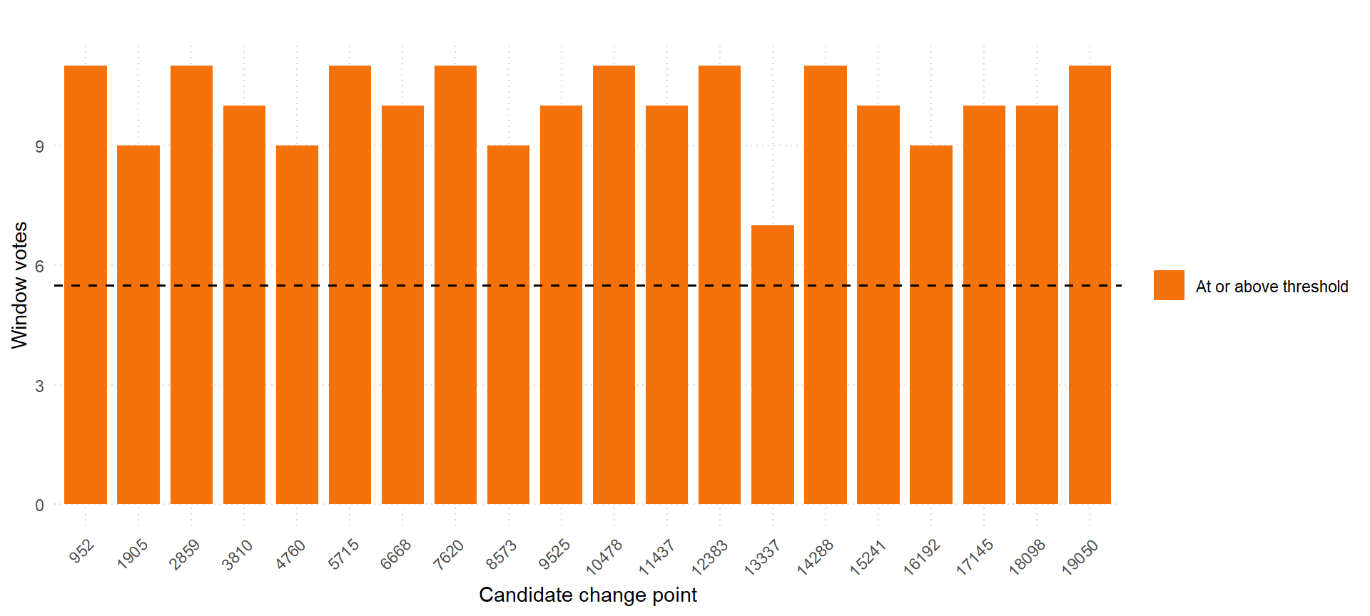
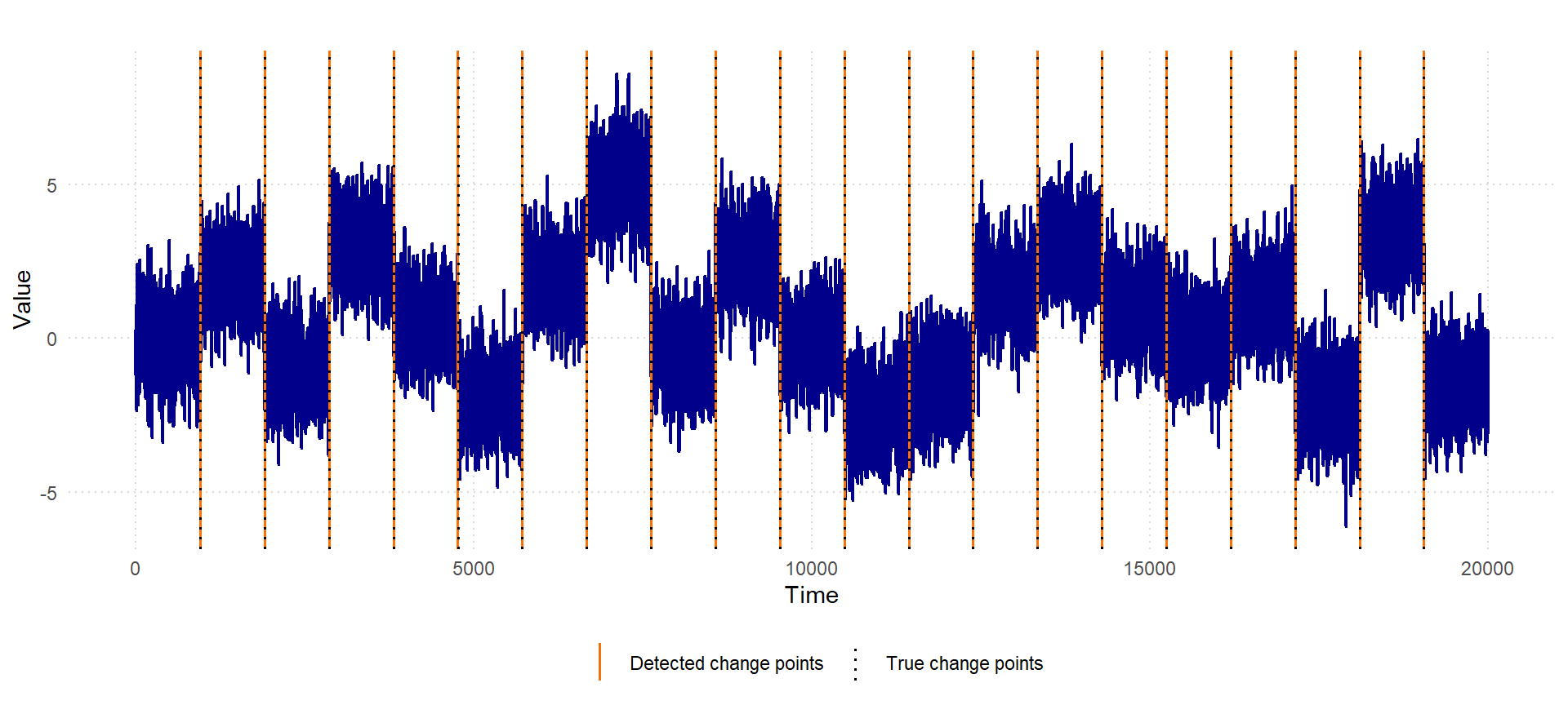
The package includes visual helpers for inspecting detected change points, window-level votes, and the overall vote scree.

vis_change_points(
  x_mean,
  fit_mean,
  true_change_points = change_points,
  x_label = "Time",
  y_label = "Value"
)

3.4 Tune the Voting Threshold

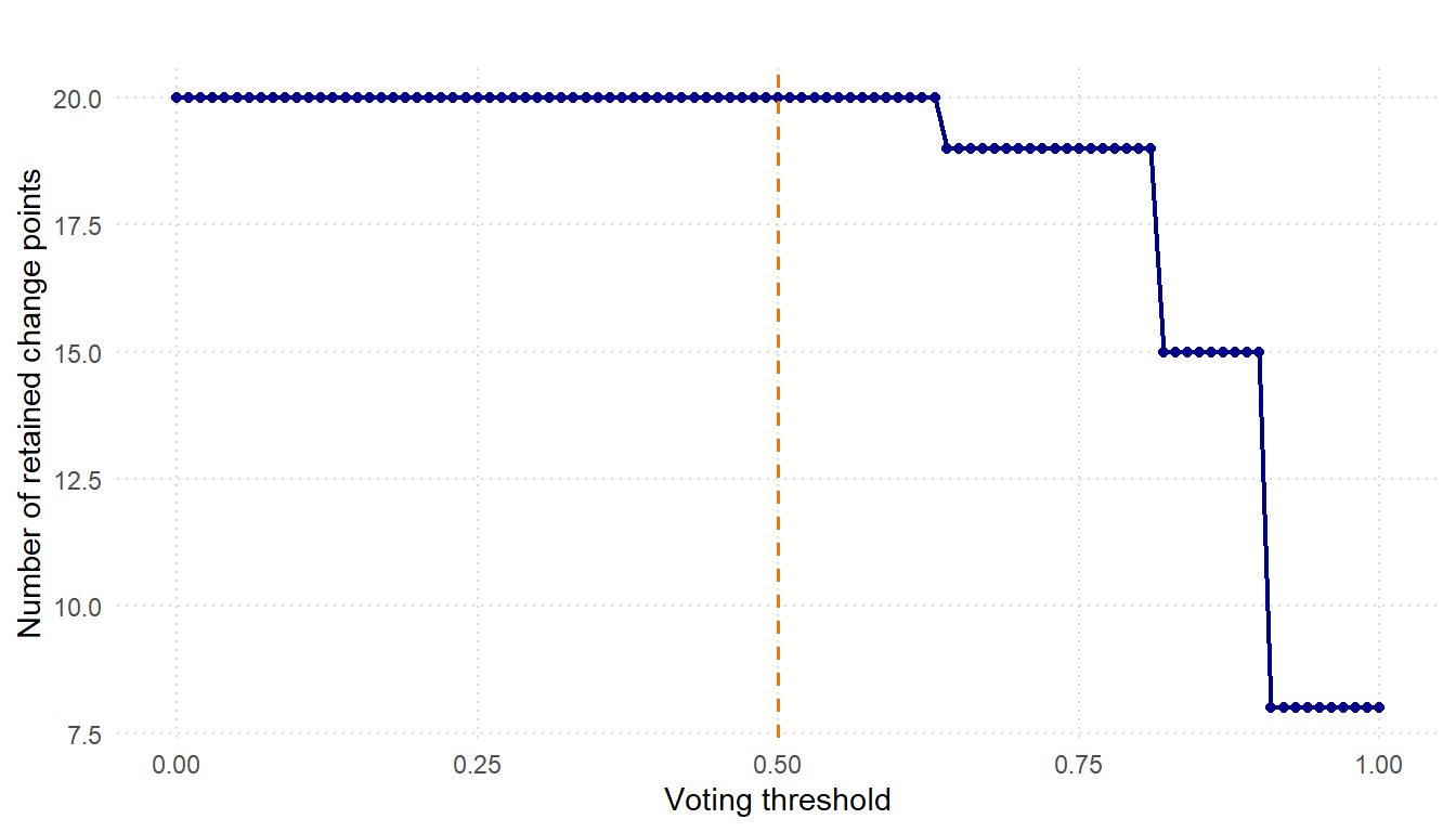
The ensemble vote threshold, vote_threshold, controls how much agreement is required across window sizes before a candidate is retained. The default value is 0.5, meaning that a candidate must be supported by at least half of the available window-level votes.

vis_vote_scree(fit_mean)

vis_window_votes(fit_mean)